The axial resolution of OCT is determined by the measurement resolution for echo time delay of light.

To derive the formula of axial resolution mathematically, I turn to Chapter 5 of the book Optical Coherence Tomography – Principles and Applications [1].

1. Monochromatic source

To start with time domain OCT, we first refer to a monochromatic complex plane wave of this form:

E_{s o}=E_{0} e^{-i k(\omega) z}

where k = 2\pi /\lambda.

When the light changes its polarization states by a mirror or biological tissues, the change can be expressed by multiplying the Jones vector and a 2 x 2 Jones matrix.

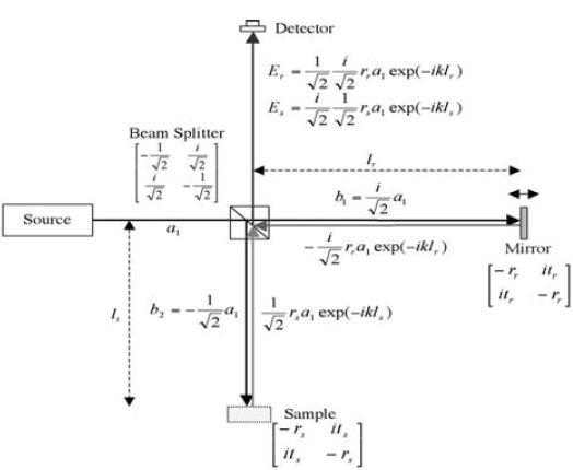
A schematic of time domain OCT (From Ref [1]).

When the light first emits from the 50/50 beam splitter, and goes into the sample and reference arm, respectively,

{E_{r1}} = \frac{1}{{\sqrt 2 }}{E_{so}}\\{E_{s1}} = \frac{i}{{\sqrt 2 }}{E_{so}}

As the light propagates, it hits the sample or the mirror, and the light beam is reflected,

{{E_{r2}} =  - {r_r} \cdot \frac{1}{{\sqrt 2 }}{E_{so}} \cdot {e^{ - ik{l_r}}}}\\{{E_{s2}} =  - {r_s} \cdot \frac{i}{{\sqrt 2 }}{E_{so}} \cdot {e^{ - ik{l_s}}}}

When the light arrive at the beam splitter for second time (from sample and reference arm), and it goes into the detector arm,

{{E_{r3}} = \frac{i}{{\sqrt 2 }}{E_{r2}} \cdot {e^{ - ik{l_r}}} =  - i \cdot \frac{{{r_r}}}{2}{E_{so}} \cdot {e^{ - i2k{l_r}}}}\\{{E_{s3}} = \frac{1}{{\sqrt 2 }}{E_{s2}} \cdot {e^{ - ik{l_s}}} =  - i \cdot \frac{{{r_s}}}{2}{E_{so}} \cdot {e^{ - i2k{l_s}}}}

The next step is interference in the detector arm, and the field becomes,

{E_D} = {E_{r3}} + {E_{s3}} = {E_R} \cdot {e^{ - i2k{l_r}}} + {E_S} \cdot {e^{ - i2k{l_s}}}

where {E_R} = - i \cdot \frac{{{r_r}}}{2}{E_{so}}, and {E_S} = - i \cdot \frac{{{r_s}}}{2}{E_{so}}.

The irradiance approaching the detector arm is obtained,

\begin{array}{l}
{I_D} =  < {E_D} \cdot E_D^* > \\
{I_D} =  < {E_R} \cdot E_R^* >  +  < {E_S} \cdot E_S^* >  + {E_R} \cdot E_S^* \cdot {e^{ - i2k{l_r} + i2k{l_s}}} + {E_S} \cdot E_R^* \cdot {e^{ - i2k{l_s} + i2k{l_r}}}\\
{I_D} = {I_R} + {I_S} + {\rm{Re}}(\gamma {(z)_{11}} \cdot \sqrt {{I_R} \cdot {I_S}}  \cdot ({e^{i2k({l_s} - {l_r})}} + {e^{i2k({l_r} - {l_s})}}))\\
{I_D} = {I_R} + {I_S} + 2{\rm{Re}}(\gamma {(z)_{11}} \cdot \sqrt {{I_R} \cdot {I_S}}  \cdot \cos (2k\Delta l))
\end{array}\label{gen-int}

where {\Delta l}={l_s}-{l_r}, and {\gamma {{\left( z \right)}_{11}}} is the degree of coherence.

\begin{array}{l}
\left| {\gamma {{\left( z \right)}_{11}}} \right| = 1,{\rm{coherent - limit}}\\
\left| {\gamma {{\left( z \right)}_{11}}} \right| = 0,{\rm{incoherent - limit}}\\
0 < \left| {\gamma {{\left( z \right)}_{11}}} \right| < 1,{\rm{partial - coherent}}
\end{array}

For TD-OCT, the reference mirror is moving with a velocity of {v_m} = \frac{{\Delta l}}{t}, and thus creates a Doppler or frequency shift {f_D} = \frac{{2{v_m}}}{\lambda } in the signal. Therefore, we obtain the irradiance,

{I_D} = {I_R} + {I_S} + 2{\rm{Re(}}\gamma {\left( z \right)_{11}} \cdot \sqrt {{I_R}\cdot{I_S}}  \cdot \cos (2\pi {f_D}t){\rm{)}}

2. Broadband light source

Next, we consider the low coherent light, or broadband light.

For the light in the detector arm, there are two components from sample and reference arm,

\begin{array}{l}
{E_R}(\omega ) \propto {E_r}(\omega ) \cdot \exp ( - i{k_r}(\omega )2{l_r} - i\omega t)\\
{E_S}(\omega ) \propto {E_s}(\omega ) \cdot \exp ( - i{k_s}(\omega )2{l_s} - i\omega t)
\end{array}

The irradiance in the detector arm is proportional to,

{I_D}(\omega ) \propto {\mathop{\rm Re}\nolimits} \{ {E_s}(\omega ) \cdot {E_r}(\omega ) \cdot \cos (\Delta \phi (\omega ))\} 

where \Delta \phi (\omega ) = 2{k_s}(\omega ){l_s} - 2{k_r}(\omega ){l_r}. Consider that we use a broadband light source,

{I_D} \propto {\mathop{\rm Re}\nolimits} \left\{ {\int_{ - \infty }^\infty  {G\left( \omega  \right) \cdot \exp \left[ { - i\Delta \phi \left( \omega  \right)} \right]d\omega } } \right\}\label{broad-int}

where {G\left( \omega \right)} is the power spectrum of the source with a central frequency of {\omega _0}.

Suppose a uniform, linear, and non-dispersive medium, k is the propagation constant in each arm and can be considered equal. Using first order Taylor expansion,

{k_s}\left( \omega  \right) = {k_r}\left( \omega  \right) = k\left( \omega  \right) = k\left( {{\omega _0}} \right) + k'\left( {{\omega _0}} \right)\left( {\omega  - {\omega _0}} \right)

Therefore,

\Delta \phi \left( \omega  \right) = 2k\left( \omega  \right)\left( {{l_s} - {l_r}} \right) = 2k\left( {{\omega _0}} \right)\Delta l + 2k'\left( {{\omega _0}} \right)\left( {\omega  - {\omega _0}} \right)\Delta l

Still, {\Delta l}={l_s}-{l_r}. Under this condition,

\begin{array}{*{20}{l}}
{{I_D} \propto {\rm{Re}}\left\{ {\int_{ - \infty }^\infty  {G\left( {\omega  - {\omega _0}} \right) \cdot \exp \left[ { - i\Delta \phi \left( {\omega  - {\omega _0}} \right)} \right]d\left( {\omega  - {\omega _0}} \right)} } \right\}}\\
{ = {\rm{Re}}\left\{ {\int_{ - \infty }^\infty  {G\left( {\omega  - {\omega _0}} \right) \cdot \exp \left[ { - i \cdot \left( {2k\left( {{\omega _0}} \right)\Delta l + 2k'\left( {{\omega _0}} \right)\Delta l \cdot \left( {\omega  - 2{\omega _0}} \right)} \right)} \right]d\left( {\omega  - {\omega _0}} \right)} } \right\}}\\
{ = {\rm{Re}}\left\{ \begin{array}{l}
\exp \left[ {i \cdot 2k'\left( {{\omega _0}} \right){\omega _0}\Delta l - i \cdot 2k\left( {{\omega _0}} \right)\Delta l} \right] \cdot \\
\int_{ - \infty }^\infty  {G\left( {\omega  - {\omega _0}} \right) \cdot \exp \left[ { - i \cdot 2k'\left( {{\omega _0}} \right)\Delta l \cdot \left( {\omega  - {\omega _0}} \right)} \right]d\left( {\omega  - {\omega _0}} \right)} 
\end{array} \right\}}\\
{ = {\rm{Re}}\left\{ \begin{array}{l}
\frac{1}{{2\pi }}\exp \left[ {i \cdot 2k'\left( {{\omega _0}} \right){\omega _0}\Delta l - i \cdot 2k\left( {{\omega _0}} \right)\Delta l} \right] \cdot \\
\int_{ - \infty }^\infty  {G\left( {\omega  - {\omega _0}} \right) \cdot \exp \left[ { - i \cdot 2k'\left( {{\omega _0}} \right)\Delta l \cdot \left( {\omega  - {\omega _0}} \right)} \right]d\left( {\frac{{\omega  - {\omega _0}}}{{2\pi }}} \right)} 
\end{array} \right\}}
\end{array}\label{new-int}

Next, we will introduce the concept of phase \Delta {\tau _p} and group delay $\Delta {\tau _g}$ as,

\left\{ {\begin{array}{*{20}{l}}
{\Delta {\tau _p} = \frac{{2k\left( {{\omega _0}} \right)\Delta l}}{{{\omega _0}}} = \frac{{2\Delta l}}{{{\omega _0}/k\left( {{\omega _0}} \right)}} = \frac{{2\Delta l}}{{{v_p}}}}\\
{\Delta {\tau _g} = 2k'\left( {{\omega _0}} \right)\Delta l = \frac{{2\Delta l}}{{1/k'\left( {{\omega _0}} \right)}} = \frac{{2\Delta l}}{{{v_g}}}}
\end{array}} \right.

where v_p and v_g are the phase velocity and group velocity, respectively. Therefore,

{I_D} \propto {\mathop{\rm Re}\nolimits} \left\{ {\frac{{\exp \left[ { - i \cdot {\omega _0}\left( {\Delta {\tau _p} - \Delta {\tau _g}} \right)} \right]}}{{2\pi }}\int_{ - \infty }^\infty  {G\left( {\omega  - {\omega _0}} \right) \cdot \exp \left[ { - i \cdot \Delta {\tau _g} \cdot \left( {\omega  - {\omega _0}} \right)} \right]d\left( {\frac{{\omega  - {\omega _0}}}{{2\pi }}} \right)} } \right\}\label{velo-int}

Now, let’s consider the light source. Since the autocorrelation function of a Gaussian source is Gaussian, it is optimal to have a source with a Gaussian spectrum to optimize OCT resolution (Answered later in this book).

G\left( {\omega  - {\omega _0}} \right) = \sqrt {\frac{{2\pi }}{{\sigma _\omega ^2}}} \exp \left[ { - \frac{{{{\left( {\omega  - {\omega _0}} \right)}^2}}}{{2\sigma _\omega ^2}}} \right]\label{gaussian}

where {\sigma _\omega } is the standard deviation of the angular frequency spectrum. We obtain,

\begin{array}{l}
{I_D} \propto {\mathop{\rm Re}\nolimits} \left\{ \begin{array}{l}
\frac{{\exp \left[ { - i \cdot {\omega _0}\left( {\Delta {\tau _p} - \Delta {\tau _g}} \right)} \right]}}{{2\pi }} \cdot \\
\int_{ - \infty }^\infty  {\sqrt {\frac{{2\pi }}{{\sigma _\omega ^2}}} \exp \left[ { - \frac{{{{\left( {\omega  - {\omega _0}} \right)}^2}}}{{2\sigma _\omega ^2}}} \right] \cdot \exp \left[ { - i \cdot \Delta {\tau _g} \cdot \left( {\omega  - {\omega _0}} \right)} \right]d\left( {\frac{{\omega  - {\omega _0}}}{{2\pi }}} \right)} 
\end{array} \right\}\\
 = {\mathop{\rm Re}\nolimits} \left\{ \begin{array}{l}
\frac{{\exp \left[ { - i \cdot {\omega _0}\left( {\Delta {\tau _p} - \Delta {\tau _g}} \right)} \right]}}{{2\pi }}\sqrt {\frac{{2\pi }}{{\sigma _\omega ^2}}}  \cdot \\
\int_{ - \infty }^\infty  {\exp \left[ { - \frac{{{{\left( {\omega  - {\omega _0}} \right)}^2}}}{{2\sigma _\omega ^2}}} \right] \cdot \exp \left[ { - i \cdot \Delta {\tau _g} \cdot \left( {\omega  - {\omega _0}} \right)} \right]d\left( {\frac{{\omega  - {\omega _0}}}{{2\pi }}} \right)} 
\end{array} \right\}
\end{array}\label{gau-int}

The following auxiliary formula can be used to reduce the above equation,

\begin{array}{*{20}{l}}
{\int_{ - \infty }^\infty  {\exp } \left( { - a{x^2}} \right)\exp \left( { - i2\pi kx} \right)dx}\\
{ = \int_{ - \infty }^\infty  {\exp } \left[ { - \frac{{a{{\left( {2\pi x} \right)}^2}}}{{4{\pi ^2}}}} \right]\exp \left[ { - i\left( {2\pi x} \right)k} \right]\frac{{d\left( {2\pi x} \right)}}{{2\pi }}}\\
{ = \sqrt {\frac{\pi }{a}\exp \left( { - \frac{{{\pi ^2}{k^2}}}{a}} \right)} }
\end{array}\label{aux-for}

It should be helpful to create corresponding relationship between components of the integral,

\left\{ \begin{array}{l}
\frac{{d\left( {\omega  - {\omega _0}} \right)}}{{2\pi }} \leftrightarrow \frac{{d(2\pi x)}}{{2\pi }}\\
\exp \left[ { - i \cdot \Delta {\tau _g} \cdot \left( {\omega  - {\omega _0}} \right)} \right] \leftrightarrow \exp \left[ { - i\left( {2\pi x} \right)k} \right]\\
\exp \left[ { - \frac{{{{\left( {\omega  - {\omega _0}} \right)}^2}}}{{2\sigma _\omega ^2}}} \right] \leftrightarrow \exp \left[ { - \frac{{a{{\left( {2\pi x} \right)}^2}}}{{4{\pi ^2}}}} \right]\\
\Delta {\tau _g} \leftrightarrow k\\
\frac{{4{\pi ^2}}}{{2\sigma _\omega ^2}} \leftrightarrow a
\end{array} \right.

We can solve the irradiance I_D,

\begin{array}{l}
{I_D} \propto {\mathop{\rm Re}\nolimits} \left\{ {\frac{{\exp \left[ { - i \cdot {\omega _0}\left( {\Delta {\tau _p} - \Delta {\tau _g}} \right)} \right]}}{{2\pi }}\sqrt {\frac{{2\pi }}{{\sigma _\omega ^2}}}  \cdot \sqrt {\frac{\pi }{{\frac{{4{\pi ^2}}}{{2\sigma _\omega ^2}}}}\exp \left( { - \frac{{{\pi ^2}\Delta \tau _g^2}}{{\frac{{4{\pi ^2}}}{{2\sigma _\omega ^2}}}}} \right)} } \right\}\\
 = {\mathop{\rm Re}\nolimits} \left\{ {\frac{{\exp \left[ { - i \cdot {\omega _0}\left( {\Delta {\tau _p} - \Delta {\tau _g}} \right)} \right]}}{{2\pi }}\exp \left( { - \frac{{\sigma _\omega ^2\Delta \tau _g^2}}{2}} \right)} \right\}
\end{array}\label{spa-int}

The equation contains two oscillatory terms. The first oscillatory term is a rapid oscillatory term. The second oscillatory term in Gaussian shape is much slower, and is the envelope of the autocorrelation function. It is this second term that primarily carries ranging information. Therefore, a source with a Gaussian frequency spectrum ideally yields a Gaussian autocorrelation function, which is critical in ranging and performing high resolution imaging [2].

3. Resolve axial resolution

The Gaussian function is,

G\left( {f - {f_0}} \right) = \sqrt {\frac{1}{{2\pi \sigma _f^2}}} \exp \left[ { - \frac{{{{\left( {f - {f_0}} \right)}^2}}}{{2\sigma _f^2}}} \right]

where {\sigma _f} = 2\pi {\sigma _\omega } is the standard deviation of the frequency spectrum. Correspondingly, the slowly oscillating component can be expressed as,

{I_{AC}} = \exp \left( { - 2{\pi ^2}\sigma _f^2\Delta \tau _g^2} \right)

The full width at half maximum (FWHM) of I_{AC} is usually indicated as the the value of axial resolution,

\exp \left( { - 2{\pi ^2}\sigma _f^2\Delta \tau _g^2} \right) = \frac{1}{2}

Therefore, we can get \Delta {\tau _g} through simple algebra,

\Delta {\tau _g} = \frac{{\sqrt {\ln 2} }}{{\sqrt 2 \pi }} \cdot \frac{1}{{{\sigma _f}}}\label{gp-v}

Since {\sigma _f} can also be expressed in terms of the wavelength, that is,

{\sigma _f} = \frac{c}{{\lambda _0^2}} \cdot {\sigma _\lambda }\label{sigma-f}

For the spectrum with a normal distribution, the relationship between FWHM and the standard deviation is (refer to FWHM on Wikipedia),

\Delta \lambda  = 2\sqrt {2\ln 2} {\sigma _\lambda }\label{delta-lambda}

We can get,

\Delta {\tau _g} = \frac{{2\ln 2}}{{\pi c}} \cdot \frac{{\lambda _0^2}}{{\Delta \lambda }}

Finally, the difference in optical group delay can be converted to the FWHM of the coherence length, which is also the axial resolution of OCT in free space,

\Delta l = \frac{1}{2}c \cdot \Delta {\tau _g} = \frac{{\ln 2}}{\pi } \cdot \frac{{\lambda _0^2}}{{\Delta \lambda }} \leftrightarrow ({\rm{Axial-Resolution}})

Reference

[1] Optical Coherence Tomography – Principles and Applications

[2] Wikipedia