2.5 Fourier-Domain Low-Coherence Interferometry
Still, the cross-correlation component is the desired part.
The FWHM of the DC artifact is only one coherence length wide, however, the signal amplitude is much higher than another two components. How to remove it ?
Record the amplitude of the spectral interferometric signal with reference reflector but no sample present, and then subtract this signal component from each subsequent spectral interferometric signal acquired.
For the autocorrelation terms, the distance between sample reflectors is much smaller than that between sample and reference mirror. How to eliminate them?
Ensure that the reference reflectivity is sufficient so that the cross-correlation terms are much larger than autocorrelation terms.
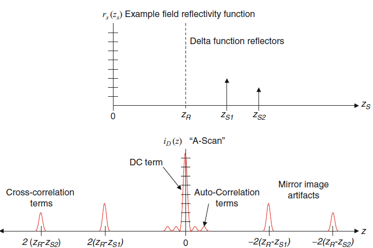
Fig.1. Illustration of the example discrete-reflector sample field reflectivity function and the A-scan resulting from Fourier-domain low-coherence interferometry (From the original book).
2.6 Time-Domain Low-Coherence Interferometry
In traditional or time-domain OCT, the wave number-dependent detector current is captured on a single receiver, while the reference delay is scanned to reconstruct an approximation of the internal sample reflectivity profile. The result is obtained by the integration over all $k$.
Here the DC offset is proportional to the sum of the reference and sample power reflectivity.
Also, the sample reflectivity profile is convolved by a cosinusoidal carrier wave modulation at a frequency proportional to the source center wave number $k_0$ and the free-space difference between reference and sample arm lengths (z_R-z_{Sn}).
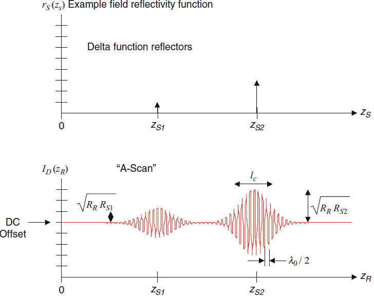
Fig.2. Illustration of the example discrete-reflector sample field reflectivity function and the A-scan resulting from time-domain low-coherence interferometry (From the original book).
2.7 Effects of Index of Refraction and Dispersion
For the dispersion constant \beta (\omega ), the zero-order term is nondispersive, and the first-order and second order can be expressed by phase velocity and group velocity, respectively.
The correction for the first-order dispersion of coherence length, the A-scan of FD-OCT and TD-OCT detector current is given in terms of phase and group indices of refraction of the sample. ==What about the second-order and higher-order dispersion?==
2.8 Practical Aspects of FDOCT Signal Processing
2.8.1 Sensitivity Falloff and Sampling Effects in FDOCT
The exponential falloff of sensitivity with depth can be understood as the decreasing visibility of higher fringe frequencies corresponding to large sample depths.
2.8.2 Artifact Removal in FDOCT by Phase Shifting
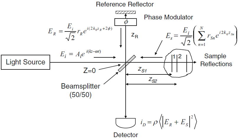
Fig.3. FDOCT interferometer with addition of variable round-trip phase delay Φ in the reference arm (From the original book).
The phase modulator can be based on electro-optic, acousto-optic, and photoelastic modulators.
Phase-shifted spectral interferograms can be acquired sequentially or simultaneously.
\begin{aligned}
I_{D}(k, 2 \phi)=& \frac{\rho}{4}\left[S(k)\left[R_{R}+R_{S 1}+R_{S 2}+\ldots\right]\right] \text { "DCTerms" } \\
&+\frac{\rho}{2}\left[S(k) \sum_{n=1}^{N} \sqrt{R_{R} R_{S n}}\left(\cos \left[2 k\left(z_{R}-z_{S n}\right)+2 \phi\right]\right)\right] \text { "Cross-correlation Terms" } \\
&+\frac{\rho}{4}\left[S(k) \sum_{n \neq m=1}^{N} \sqrt{R_{S n} R_{S m}} \cos \left[2 k\left(z_{S n}-z_{S m}\right]\right]\right. \text { "Auto-correlation Terms" }
\end{aligned}
2.8.2.1 Stepped Phase-Shifting Interferometry Approach
Set the round-trip phase delay {\rm{2}}\phi {\rm{ = }}\pi and {\rm{2}}\phi {\rm{ = 0}}, and do the subtraction, the DC and autocorrelation terms will be eliminated.
To remove the complex conjugate artifact, at least two spectral interferograms with noncomplementary phase delays, for example, {\rm{2}}\phi {\rm{ = }}\pi/2 and {\rm{2}}\phi {\rm{ = }3\pi/2}.
2.8.2.2 Quadrature Projection Phase Correction
2.9 Sensitivity and Dynamic Range in OCT Systems
Sensitivity/signal-to-noise ratio: the minimum detectable reflected optical power compared with a perfect reflector.
Dynamic range: the range of optical reflectivities observable within within a single acquisition.
2.9.1 SNR Analysis for Time-Domain OCT
Shot-noise is the fundamental limiting noise for optical detection. In OCT detection, design approaches for obtaining shot-noise-limited operation are usually applied.
The SNR is proportional to the detector responsivity \rho and to the power returning from the sample, but is independent of the reference arm power level.