乐鱼(原名:广东省佛山水泵厂有限公司),创立于1954年,是一家集研发、生产、销售、服务于一体的综合性泵及成套装备公司,被认定为高新技术企业、中国机械工业500强、中国机械工业企业核心竞争力优秀企业、广东省专精特新中小企业、广东省创新型中小企业和广东省百强民营企业。
公司现有员工1200多人,建有三个生产厂区,分别位于佛山三水白坭工业园、乐平工业园和遵义绥阳高新技术产业园,总占地29.8万平方米,建筑面积为14万平方米,生产设备先进,手段齐全,拥有从模具制造、铸造、焊接、热处理、加工、组装、试验等全工序过程。
公司专注于泵及成套装备的应用研究,为用户提供技术解决方案,拥有一支以高级工程师为核心的专业技术团队和一支高素质的技工队伍。长期以来,通过不断的科研投入、技术创新、产学研合作,推动了公司的新产品开发和技术进步,形成了公司的核心技术和独特专长。
公司已通过质量管理体系(ISO9001 )、环境管理体系(ISO14001 )及职业健康安全管理体系(ISO45001) 认证。
公司营销及服务网络遍及全囯各地,在海外设有子公司。产品被认定为制造业单项冠军产品、广东省名牌产品,广泛应用于石油、化工、电力、造纸、煤炭、轻工、供水、节能、环保等行业,并以高效节能、运行可靠而享誉海内外市场。

质量至上,追求一流品质、满足并超越客户期望
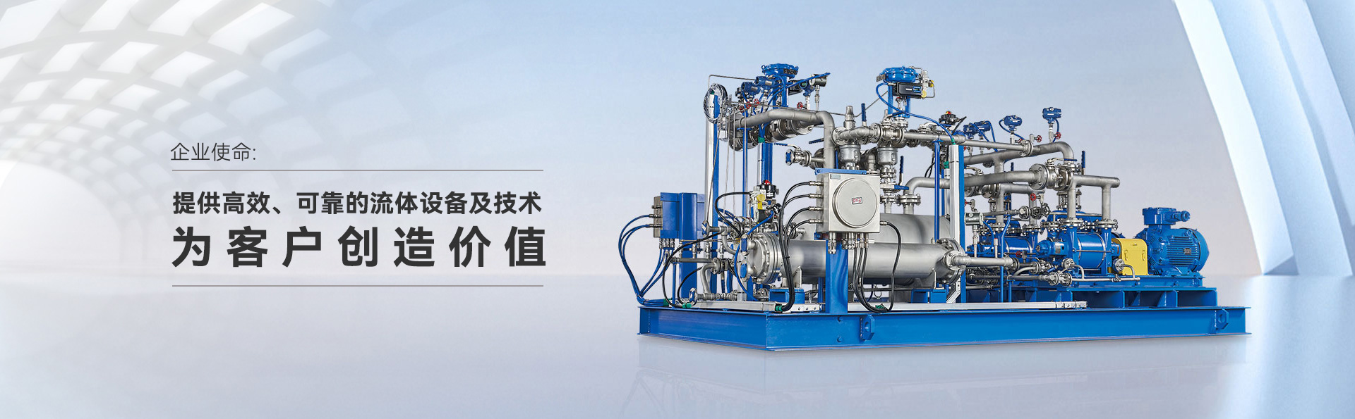
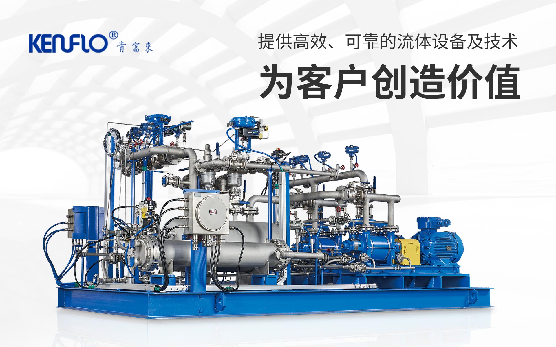
提供高效、可靠的流体设备及技术,为客户创造价值
厚道、诚信、感恩、共赢
实时更新肯富来最新动态,了解肯富来文化
09
2024.09
各位股东:2024年9月27日08:45在本公司会议室召开2024年第一次临时股东大会,相关资料详见附件。特此公告。附件资料:2...
26
2024.06
2024年6月12日至6月13日,广东省能源领域大规模设备更新和节能改造技术专题对接会在广州顺利召开。此次会议由广东省能源局、人民银行广东省...
26
2024.06
6月10日至14日,世界知名的ACHEMA化工流程展在德国法兰克福展览中心举行,该展会吸引了来自世界各地的参展商和专业观众。作为中国化工泵的...
乐鱼